Load microscopy data
Microscopy Nodes uses the same loading workflow for fluorescence, dense EM, segmentations, and time series. What changes is the representation and visualization chosen for each channel.
1. Point to your data
-
Delete everything in the scene with
AandX -
In the Scene Properties panel, find the Microscopy Nodes panel.
-
Provide the path to your data set:
local TIFF file (preferably imagej-tif, but others work)
OME-Zarr URL
local OME-Zarr folder
For local files, you can use the file explorer .
With OME-Zarr URLs/folders, copy the address directly into the field. OME-Zarr links are not clickable. If the metadata does not populate, check out our tips for troubleshooting OME-Zarr.
Example OME-Zarr datasets:
- https://s3.embl.de/microscopynodes/RPE1_4x.zarr ; Showing expansion microscopy of an RPE1 cell with cytoskeletal elements stained
- https://s3.embl.de/microscopynodes/FIBSEM_dino_masks.zarr ; Showing a dinoflagellate FIB-SEM dataset with segmentations
- The Image Data Resource OME-Zarr archive. Some may not work.
2. Select scale (optional)
Microscopy Nodes automatically selects the smallest scale of data available.
If the source data is larger than 1 GiB per timepoint, Microscopy Nodes automatically offers additional downscaled versions. This applies to both TIFF and OME-Zarr sources. For OME-Zarr, any multiscale levels already stored in the source are shown as well.
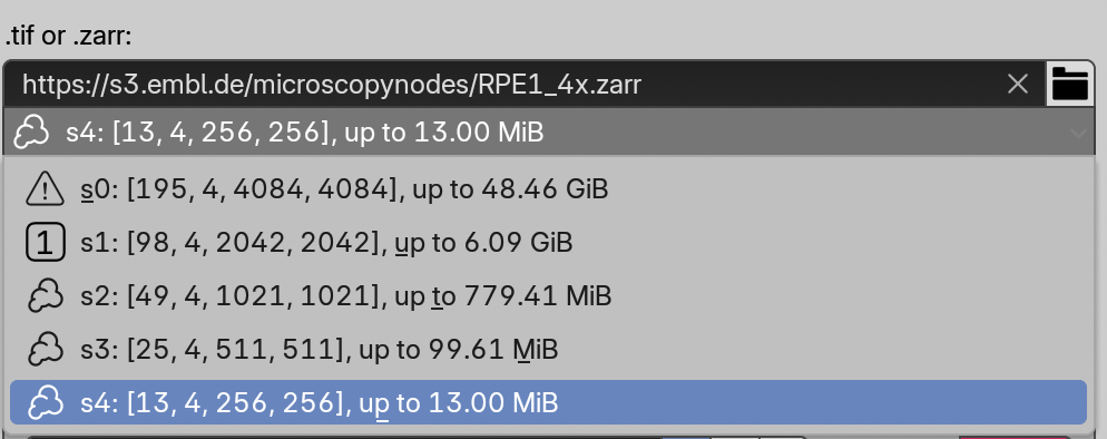
Any scale with a volume icon will easily work in any part of Blender. The 1 icon is of a size where a single channel will definitely work. For larger datasets, check out the large data tutorial.
3. Check metadata
The metadata populates automatically from the file:
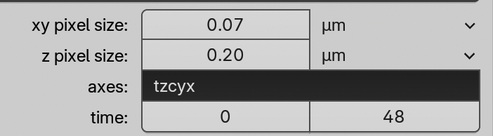
This contains:
- Pixel Sizes
This may be truncated in the view, up to 6 decimal places are used.
- Pixel Units
Å, nm, µm, mm, or m
- Axis order
A piece of text such as 'tzcyx'. number of letters needs to match the number of axes. Allows remapping of axis order by editing the text field.
- Time (only if time axis exists)
Start and end frame, allows you to clip the time axis before loading.
4. Set channels
Next we see the channel interface:
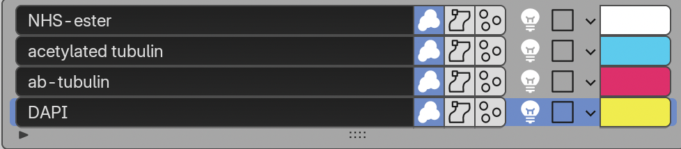
From left to right:
- Channel name (editable)
- Visualization types:
- Volume
- Surface
- Labelmask
- Emission on/off
- Colormap type:
- Single Color
- Linear
- Diverging
- Categorical
- Color Picker ( if )
The Visualization type defines which objects will be loaded. If none are clicked in a channel, this channel will not be loaded.
When loading with Emission on , the objects of this channel will by default emit light. If this is off , they will reflect/scatter light from the scene or background.
The Colormap choice gives basic options for color before loading. If Single Color is picked, the colormap will be linearly black -> color picked in the color picker.
Defaults can be changed in the preferences.
Labelmasks
Labelmasks expect an array with separate integer values per object. If it gets a data channel, it will try to still split it into separate objects
5. Extra import settings (optional)
These settings are below the Load button. Most users can leave them at their defaults for a first load.

The panel is ordered as follows:
- On load – Scene
- sets the world color to white when any non-emissive channel is loaded, or black when all loaded channels emit light.
- applies Microscopy Nodes' responsive render defaults. It turns itself off after a successful load so later loads do not overwrite settings you have changed.
- On load – Slicing
- Geometry adds a Mask Grid or Mask Mesh node to each loaded data object. This supports arbitrary masks and sparse reloading, but its voxelized boundaries can look stepped.
- Shader clips the rendered material with the Slice Cube. It gives a clean box boundary but does not mask the underlying data.
-
Data Storage chooses where converted VDB and mesh cache files are written:
-
Temporary (Default)
Puts the data in a temporary file, you can check the temporary path in the preferences
- Path
Gives a field to put in a location.
- With Project
Will create a folder next to the project location. Requires that the project is saved
The storage choice and default slicing mode persist in the add-on preferences.
6. Set coordinate scale and location
The scale and location controls sit below the extra-settings box. They are responsive controls, not one-time loading options: changing either one updates an already loaded dataset immediately.

Microscopy scale → Blender scale converts the physical units of the dataset into Blender meters. Auto chooses a practical scene size. Manual choices are available for nm, µm, mm, and m, with output scales in meters, decimeters, or centimeters; nm → cm (Molecular Nodes) matches Molecular Nodes conventions.
defines the input location:
XY CenterXYZ CenterOrigin
The location is applied through the dataset's holder, so XY Center, XYZ Center, and Origin reposition the whole hierarchy without changing the data coordinates inside it.
7. Load
Press the big Load button to load a dataset
Switch the viewport to Material Preview or Rendered Preview to see volume data. The resulting hierarchy contains a holder, the selected data objects, an Axes object, and a Slice Cube.
Next, use Adjust color, contrast, and opacity to make the signal readable, or see How Microscopy Nodes works for an overview of the generated scene.
8. Reload data or settings
Point the Reload field to an existing Microscopy Nodes holder to update it instead of creating a new hierarchy.

- Update data replaces the underlying data, scale, or selected time range.
- Update settings reapplies channel representations, colors, emission choices, and other loading settings.
Turn off Update settings when replacing a small working scale with final high-resolution data while retaining shader edits. Turn off Update data when only the channel configuration needs to change.
For regional high-resolution loading, continue with Large datasets and sparse reloading.